Every digital communication system eventually runs into the same question: how do you send information without wasting bandwidth on data the receiver could have guessed anyway? That question is exactly what led engineers to move beyond basic Pulse Code Modulation and develop Differential Pulse Code Modulation, better known as DPCM.

If you're studying digital communication, telecommunications engineering, or signal processing, DPCM is one of those topics that shows up early and then quietly resurfaces later in more advanced coding schemes. Understanding it properly now saves you a lot of confusion when you get to ADPCM, speech codecs, and even parts of image compression theory.

This guide covers what DPCM is, why it exists, how the encoding and decoding process actually works, its strengths and weaknesses, and how it compares with related techniques. By the end, you should be able to explain DPCM to someone else, not just recognize the acronym.

What Is DPCM?

Differential Pulse Code Modulation is a signal encoding technique used in digital communication. Instead of encoding the full amplitude of each signal sample, as standard Pulse Code Modulation does, DPCM encodes the difference between the current sample and a value predicted from previous samples.

The logic behind it is straightforward once you sit with it for a moment. Most real signals, especially speech, don't change randomly from one instant to the next. They drift, rise, and fall in patterns. If you can predict where a sample is likely to land based on what came before it, you only need to transmit how far off that prediction was, not the entire value from scratch.

That "how far off" number is usually small. Small numbers need fewer bits. Fewer bits mean lower bandwidth requirements for the same signal, or better quality within the same bandwidth budget. That's the entire value proposition of DPCM in one sentence.

The Problem DPCM Was Built to Solve

Standard PCM samples an analog waveform at fixed intervals and converts each sample into a binary code using a set number of bits, commonly 8 bits per sample for telephone-grade voice. That gives good fidelity, but it comes at a cost. A 64 kbps PCM voice stream, for example, treats every single sample as new, independent information, even though consecutive voice samples are almost always closely related to each other.

This is redundancy, plain and simple. And in any bandwidth-limited system, whether it's a telephone trunk line or a satellite link, redundancy is something engineers actively try to eliminate. DPCM was developed specifically to attack this redundancy by exploiting the correlation between neighboring samples instead of ignoring it.

How DPCM Works, Step by Step

Here's the sequence a DPCM system follows, broken down without the jargon overload:

1. The analog input signal is sampled at a fixed sampling rate, just like in standard PCM.

2. A predictor, using one or more previously reconstructed samples, estimates what the current sample's value should be.

3. The system calculates the error, meaning the difference between the actual sampled value and the predicted value.

4. That error value, which is typically much smaller in magnitude than the raw sample, is quantized using fewer bits.

5. The quantized error is transmitted (or stored) instead of the original sample value.

6. On the receiving side, the decoder uses the same prediction rule, adds the received error back to its own predicted value, and reconstructs an approximation of the original sample.

7. This reconstructed sample then becomes part of the input the predictor uses for the next cycle, keeping encoder and decoder in sync.

That feedback loop, where the decoder's own output feeds back into future predictions, is what makes DPCM self-correcting in normal operation, and also what makes it vulnerable to error propagation when something goes wrong.

The Role of the Predictor

The predictor is really the brain of the whole system. A DPCM scheme is only as good as its ability to guess the next sample accurately, because a bad guess means a large error signal, and a large error signal defeats the entire purpose of using fewer bits.

Simple DPCM systems often use a first-order predictor, where the prediction for the current sample is just the previous reconstructed sample, sometimes with a scaling coefficient applied. More sophisticated systems use linear predictors that combine several previous samples, each weighted according to how strongly it correlates with the current one.

This is also the exact point where DPCM evolves into Adaptive DPCM. Instead of using fixed prediction coefficients and a fixed quantizer step size, ADPCM adjusts both dynamically based on recent signal behavior, which is part of why ADPCM generally performs better on real-world speech than plain DPCM.

Quantization in DPCM

Once the error signal is calculated, it still needs to be converted into a digital code, and that's where quantization comes in. Because the error signal has a much smaller dynamic range than the original sample, it can be represented accurately with fewer quantization levels, which directly translates into fewer bits per sample.

There's a trade-off here worth understanding. Coarser quantization saves more bits but introduces more quantization noise into the reconstructed signal. Finer quantization preserves quality but reduces the bit-rate savings DPCM is designed to deliver. Engineers tune this balance based on the application, whether that's toll-quality telephone speech or lower-fidelity telemetry data where some quality loss is acceptable.

Block Diagram Logic: Transmitter and Receiver

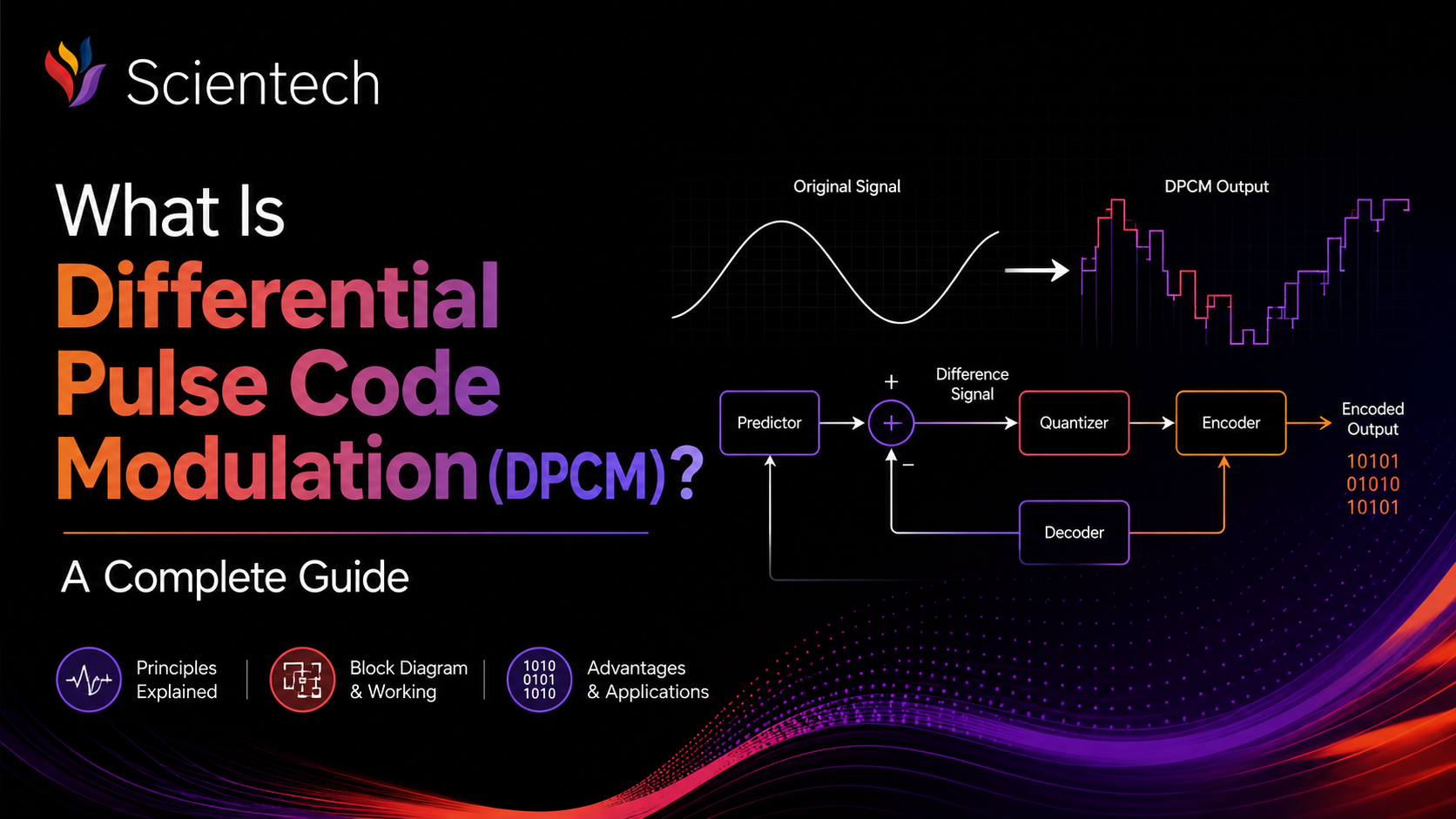
On the transmitter side, the core blocks are: sampler, predictor, subtractor (which computes the error between actual and predicted sample), and quantizer/encoder, which prepares the error signal for transmission over the channel.

On the receiver side, the blocks mirror the transmitter: a decoder recovers the quantized error, an identical predictor generates its own estimate, and an adder combines the received error with the prediction to reconstruct the sample. That reconstructed value also loops back into the predictor, exactly as it does on the transmitter side, so both ends stay synchronized sample after sample.

This symmetry between transmitter and receiver logic is one of the more elegant aspects of DPCM, and it's a big part of why lab trainers built around this technology are so effective for teaching. Watching both sides operate side by side, with the same predictor logic running independently but in step, makes the concept far more intuitive than reading it off a textbook diagram.

Advantages of DPCM

• Lower bit rate for the same signal quality, since the error signal typically requires fewer bits than the raw sample amplitude.

• Better bandwidth utilization, which matters directly in telephony, satellite links, and other channel-limited systems.

• Strong performance on correlated signals, particularly speech and many types of sensor or telemetry data.

• A relatively simple architecture compared to some other compression techniques, given the meaningful savings it provides.

Disadvantages and Practical Limitations

• Error propagation: because decoding depends on previously reconstructed samples, a single transmission error can affect several subsequent samples before the system stabilizes again.

• Predictor sensitivity: the entire scheme's efficiency depends on how well the predictor models the actual signal. A predictor tuned for voice won't necessarily perform well on a different type of data.

• Diminishing returns on uncorrelated signals: if the signal doesn't have meaningful sample-to-sample correlation, DPCM offers little advantage over plain PCM.

• Accumulated quantization error: since quantized error feeds back into the prediction loop, small quantization inaccuracies can build up over time if the system isn't well designed.

Where DPCM Is Used Today

• Telephony systems, where reducing the bit rate of digitized voice has direct cost and bandwidth benefits.

• Speech compression, particularly in earlier codec designs that laid the groundwork for today's more advanced voice compression standards.

• Telemetry and sensor networks, where readings often change gradually and differential encoding reduces the data volume that needs to be transmitted or stored.

• Foundational concepts in image and video compression, where predicting a pixel or block from neighboring data and encoding only the residual traces its logic directly back to DPCM.

Studying DPCM Practically

Reading about predictors and quantizers gets you partway there, but DPCM is one of those topics that really sinks in once you watch it happen. Seeing an actual differential waveform generated at the transmitter, then watching a receiver reconstruct the original signal from that waveform, connects the theory to something tangible.

This is exactly why dedicated communication lab trainers exist. A trainer like the Scientech 2113 DPCM Trainer, for instance, includes an onboard DPCM transmitter and receiver, a signal generator block, audio input and output processing circuits, and clock and control sections, allowing students to trace the entire data and control signal flow directly. Instead of just accepting that "DPCM reduces bit rate by encoding the difference between samples," students can actually observe that difference being generated, quantized, transmitted, and reconstructed in real time on an oscilloscope.

For engineering colleges, communication labs, and technical training centers, this kind of hands-on exposure tends to make DPCM, and later ADPCM, click far faster than lecture slides alone ever could.

Conclusion

DPCM is built on a deceptively simple insight: if you can predict something reasonably well, there's no reason to keep re-transmitting it in full. By encoding only the error between a signal's actual value and its predicted value, DPCM manages to cut down the bit rate needed for correlated signals like speech, without sacrificing the ability to reconstruct the original waveform accurately at the receiver.

Its limitations, particularly error propagation and its dependence on a well-tuned predictor, are exactly what pushed engineers toward adaptive versions like ADPCM. But those later techniques only make sense once you understand the prediction-and-difference logic DPCM introduced first. Whether you're working through the math in a textbook or tracing waveforms on a trainer like the Scientech 2113 in a lab session, the goal is the same: understanding that in digital communication, what you don't have to send is often just as important as what you do.

Learn what DPCM (Differential Pulse Code Modulation) is, how it works, and why it's more efficient than PCM. Covers predictors, ADPCM, and uses